The optional module to calculate proximity function by Monte-Carlo method for multilayered substrates is created

May 25, 2009

The optional module to calculate proximity function for multilayered substrates is created. The calculated distribution of the absorbed energy (dose) in a resist is fitted by two Gaussians which parameters vary with depth. A new parameter - ₀, added to proximity function, allows to consider dose changes with resist depth. The data calculated by Monte-Carlo method, along with former experimental data, are used now as Recommended Parameters at exposure, proximity effect correction and simulation of resist development procedures.

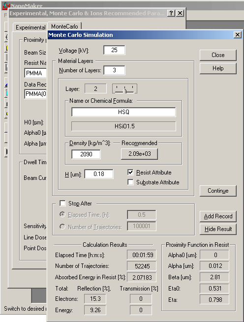
The dialog is used to set initial parameters and to run software for calculation of absorbed energy distribution after scattering of electrons in multi-layer target. Incident electron beam falls down (perpendicular to XY plane of layers) and has zero size (diameter). Numbering of layers starts on surface from a point of beam falling and proceeds deep into target. Topmost layer has number 1, last deepest layer has maximal number. Up to 20 layers can be introduced.
Monte Carlo method is used for simulation of a large number of electron trajectories. The algorithm uses Rutherford scattering at a screened nucleus and continuous-slowing-down approximation for energy loss along an electron trajectory [1]. Lost energy is accumulated in cells of a calculation grid. The grid has cylindrical symmetry in XY plane with center at axis of electron beam and grid is irregular along radius and Z direction. This speeds up calculation allowing 50000 trajectories per 2 min (Voltage=25 kV; PMMA resist H=0.5 m; Si substrate) on Intel Core Duo CPU. Such quantity of trajectories usually is sufficient for proximity parameters calculation.

One layer in the target should be marked as resist one. Energy distribution in the layer is the sought proximity function I(x,y,z) for proximity effect correction and for resist development simulation.

Where = 3.1415…. Energy distribution accumulated in the calculation grid is fit by the formula using linear approximation for (z) (₀=(H) on top of resist surface, - on bottom of resist surface). ²(z)= ₀²+( ²-₀²)*( 1-z/H )³, where z- distance from resist bottom. Five parameters: ₀, , , ₀, define proximity function for Proximity Simulation. Three parameters: , , set proximity function for Proximity Correction.

[1] L. Reimer "Scanning Electron Microscopy. Physics of Image Formation and Microanalysis" Second Edition Springer Series in Optical Sciences Vol. 45, 1998

Back to News